BLUF: Filter sensor signals before reducing their sample rate. Keeping every fourth observation can move a real high-frequency vibration into a false low-frequency feature. Define the retained band, anti-aliasing attenuation, timing assumptions and causal filter state as part of the model’s feature contract—not as an undocumented storage optimisation.
This article executes a synthetic two-tone example, not a bearing-fault benchmark. Reducing 2,000 samples per second to 500 folds an unfiltered 420 Hz component to 80 Hz. An explicit low-pass FIR prevents that contamination in the example, but introduces delay and deliberately discards information. If the diagnostic signal lives in the discarded band, the downsampling decision itself is wrong.
Which information are you allowed to discard?
Start with the physical measurement and the maintenance decision. Identify the useful frequency band, sensor and acquisition bandwidth, analogue anti-aliasing path, maximum plausible out-of-band amplitude, units and clock provenance. A slower trend signal and a bearing-vibration waveform are not interchangeable just because both arrive as numeric arrays.
There are two separate boundaries. Before analogue-to-digital conversion, the acquisition system must control frequencies that would alias at its original sample rate. After acquisition, a digital low-pass filter can protect a subsequent rate reduction. It cannot uniquely recover information already aliased by the ADC. Verify the actual sensor, analogue front end and ADC configuration rather than assuming a Python routine repairs the acquisition chain.
For uniformly sampled real signals, the output Nyquist frequency is half the output sample rate. That is a limit, not a recommended passband edge. A practical finite filter needs a transition band. In this fixture the retained band is 0–100 Hz, the transition is 100–200 Hz, and attenuation is required from 200 Hz onward, below the new 250 Hz Nyquist boundary. Those are illustrative design choices, not plant defaults.
Extend the existing industrial data contract with this signal-processing meaning. “Acceleration in the correct unit” is insufficient if one producer sends an unfiltered waveform and another sends a bandwidth-limited feature stream under the same name.
An executed two-tone fixture
The input is x(t) = sin(2π·50t) + 0.6·sin(2π·420t), sampled uniformly at 2,000 Hz for eight seconds. Both components are below the original Nyquist limit. Downsampling by four produces 500 Hz. The folded frequency is abs(((f + Fs_out/2) modulo Fs_out) − Fs_out/2): for 420 Hz, the result is 80 Hz. The alias may have a different phase; a spectral peak at 80 Hz does not identify the original physical source.
The run used NumPy 2.4.6 and SciPy 1.17.1. Its amplitudes are synthetic, dimensionless and not calibrated sensor units. Measurements below use the interior interval from 1 s inclusive to 7 s exclusive, avoiding the filter boundaries. Sinusoidal amplitudes come from least-squares sine/cosine fits at 50 and 80 Hz; RMS is the square root of the mean squared output over that same interval. The spectrum uses that six-second rectangular window, which contains whole cycles of the fixture tones.
Naive slicing x[::4] retained an 80 Hz amplitude of 0.600000. Its RMS was 0.824621, compared with 0.707107 for the desired unit-amplitude 50 Hz sine alone: a 16.62% inflation relative to that deliberately band-limited target. This is not evidence that total wideband vibration decreased in the physical machine. It demonstrates that a feature intended to represent the retained band now contains folded energy.
Both filtered paths produced an 80 Hz amplitude of approximately 8.47×10⁻⁷, a 50 Hz amplitude of 1.000033 and RMS 0.707130 in the interior interval. Agreement in stationary amplitude does not mean their timestamps or online availability agree.
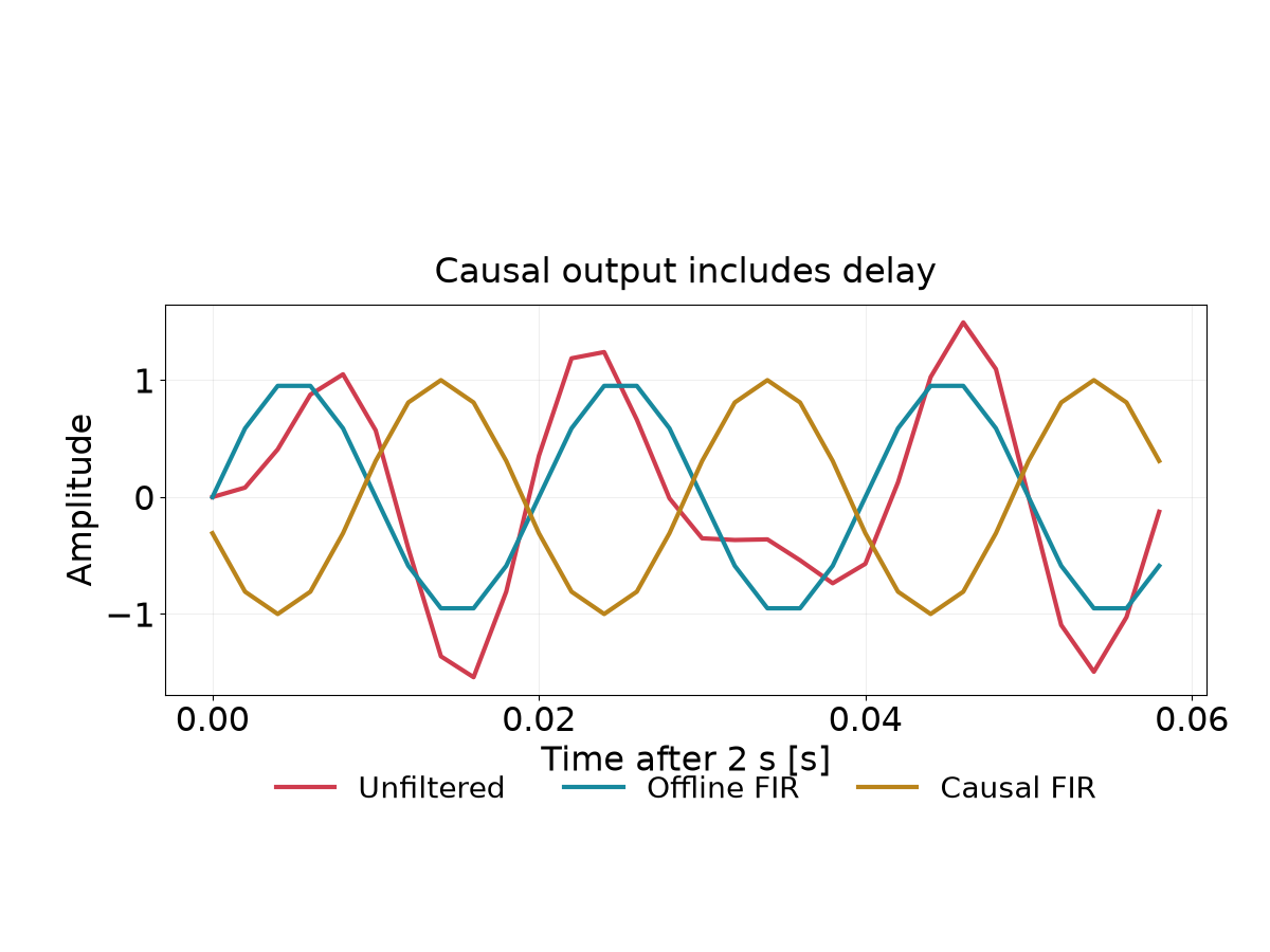
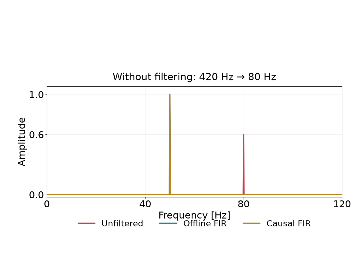
The upper plot keeps the output timestamps unchanged so the causal delay remains visible. The lower plot shows the false 80 Hz peak without filtering; the offline and causal filtered spectra overlap. These plots come from the executed arrays, not an illustrative performance chart.
Make the filter specification reproducible
The required stopband attenuation was at least 80 dB. We requested a more conservative 90 dB Kaiser design because its order estimate is empirical. The kaiserord documentation explicitly demonstrates that the requested attenuation can be missed at a stopband lobe. A design call is not an acceptance test.
The exact recipe is n, beta = signal.kaiserord(90, 100/(2000/2)); make n odd; then h = signal.firwin(n, 150, window=('kaiser', beta), fs=2000). This produces 117 coefficients with beta 8.95926. The firwin contract defines a linear-phase FIR and treats its scalar cutoff as the half-amplitude point. Here 150 Hz is the centre of the transition, not the promised passband edge.
The run saved all coefficients as one-column decimal text using %.18e. Its SHA-256 is 127d58fc76ba526b349c67d27a7922aeec8a81e4fe80c7289a95d959aad0609b. Regenerate the coefficients with the pinned runtime and retain the actual array with the release; a hash alone does not supply an implementation. Check the deployed numeric precision and coefficient representation separately.
Evaluating signal.freqz(h, worN=131072, fs=2000) gave a minimum sampled stopband attenuation of 89.57 dB from 200 Hz upward, and 0.000541 dB peak-to-peak passband ripple through 100 Hz. This dense-grid result exceeds the fixture’s 80 dB target; it is not a formal bound between every frequency-grid point or proof for fixed-point hardware. Choose attenuation from the largest credible rejected component and allowable residual feature error, not from these convenient numbers.
Decision table: offline and streaming are different contracts
| Path | What the example does | Timing and boundary cost | Appropriate decision |
|---|---|---|---|
| Naive stride | x[::4]; false 80 Hz amplitude 0.6 | No anti-aliasing protection | Reject unless upstream band-limiting is independently established |
| Offline FIR | resample_poly(x, 1, 4, window=h) | Centred output; zero padding at record edges | Retrospective analysis with an explicit boundary policy |
| Causal FIR | lfilter(h, [1.0], x), then global stride | 29 ms group delay; startup history required | Streaming features with state and timestamp accounting |
| IIR alternative | Design low-pass SOS, then sosfilt and stride | Frequency-dependent delay and longer transient policy | Consider when compute or delay budgets justify a different response |
SciPy’s resample_poly documentation describes upsampling, a low-pass FIR and downsampling, with boundary assumptions. The fixture passes its own symmetric coefficients and uses constant zero padding. With up=1, the filter is designed at the original input rate. Other rational ratios require designing at the documented upsampled rate; do not reuse this coefficient array unchanged.
The convenience function decimate also filters before downsampling and expects equidistant samples. Its zero_phase setting changes phase handling. Do not equate a zero-phase offline result with zero-latency causal streaming, or call independent chunk-level resampling and assume the boundaries disappear.
Preserve state and decimation phase across chunks
The streaming fixture uses the FIR through lfilter. Start with zi = zeros(len(h) − 1). For each chunk, compute y, zi = lfilter(h, [1.0], chunk, zi=zi). Carry the returned state into the next contiguous chunk. With offset equal to the number of input samples already processed, emit y[(-offset) % 4::4], then increase offset by len(chunk). Keep state separately for each sensor and continuous acquisition segment.
The test deliberately uses 137-sample chunks, not a multiple of four. Comparing the concatenated output with filtering the entire signal and then slicing gave a maximum absolute difference of 6.66×10⁻¹⁶; the acceptance tolerance was 10⁻¹². A negative control that reset the filter for every chunk produced a maximum error of 1.039164 against the continuous result. Preserving only filter state is insufficient: resetting the stride phase also changes the output time grid.
For this symmetric 117-tap FIR, group delay is (117 − 1)/(2·2000) = 29 ms. Its causal support spans 58 ms. Do not confuse these numbers: startup validity depends on missing history across the full support, whereas group delay describes the phase response. In this fixture, zero-initialised startup differed by about 1.00524 from a hypothetical indefinitely running delayed 50 Hz sine. Exclude startup-contaminated windows or supply validated history; zero initial state is an assumption, not observed sensor history.
Retain both the represented signal time and the time the result became available. Subtracting group delay from a timestamp does not make the result available earlier. Buffering, transport, computation and the feature window add their own costs. If you choose an IIR instead, sosfilt exposes initial and final state for cascaded second-order sections; its delay is generally frequency-dependent, unlike this symmetric FIR. That alternative was not benchmarked here.
Timing faults should invalidate a segment, not invent samples
The fixture’s guard rejects a deleted sample, a rate change to 1,800 Hz and injected timestamp jitter. It checks consecutive intervals against 1/2000 s with a 1 ns absolute tolerance and zero relative tolerance, including continuity between chunks in a deployed implementation. That strict numerical tolerance tests generated timestamps only; it is not a realistic universal plant-clock specification.
For production, define tolerances from the acquisition clock and timestamp resolution. Inspect source sequence numbers and source time, not network arrival spacing. Reorder only within an explicit policy, reject duplicate or reversed samples, and decide whether a gap ends the segment. A new sample rate requires a compatible filter, new phase mapping and a versioned feature contract. Never silently feed irregular timestamps into an algorithm that assumes a uniform grid.
Interpolation is a separate modelling decision with its own bandwidth and missingness assumptions; it cannot recover unknown high-frequency content. Keep this question separate from late-data feature finalisation: a watermark governs when observations may revise a result, not whether their sampling preserved frequency information.
Feature-contract release checklist
1. Freeze input/output rates, physical retained band, transition band, maximum out-of-band amplitude and residual-error budget; retain acquisition anti-aliasing evidence.
2. Version the coefficient array, numeric precision, implementation and response test. Distinguish offline centring from causal filtering and declare padding, startup exclusion and gap recovery.
3. Persist filter state and global decimation phase with the source offset. Test checkpoint recovery against uninterrupted output before claiming restart continuity.
4. Bind window duration, alignment, overlap, taper, units, feature formula and represented/available timestamps to the same contract. The six-second rectangular window here is an experiment, not a recommended maintenance window.
5. Test stopband and passband edges, chunk boundaries, startup, gaps, clock jitter, rate changes and sensor replacements. The executed fixture covers synthetic chunk continuity, a reset-state negative control and timing rejections; actual ADC behaviour, crash recovery and fixed-point deployment still need integration tests.
6. Replay training features through the same causal path as serving. Follow the availability-aware maintenance backtest contract: centred filtering must not smuggle future observations into a claimed online decision.
The useful boundary of this result
Filtering trades storage and downstream compute against lost bandwidth, processing cost and delay. Shorter filters or tighter transitions change those trade-offs; a smooth-looking plot does not establish a safe choice. The synthetic experiment proves neither bearing-fault accuracy nor avoided downtime. Keep inference advisory and outside the safety-control path.
For an implementation review, bring one sensor’s acquisition specification, a raw contiguous waveform, source timestamps and the intended feature definition. I can help turn them into a versioned resampling contract, executable rejection tests and a latency budget. The first decision is whether the proposed lower-rate stream still contains the physical evidence the maintenance question needs.