
BLUF: Equal sensor timestamps do not prove simultaneous acquisition. Before joining industrial features, map both source clocks into a declared reference domain, retain a defensible uncertainty interval and accept a pair only when its worst-case separation fits the feature’s physical tolerance. Separate definitely misaligned pairs from indeterminate ones. Unknown acquisition semantics must invalidate the input rather than become a precise-looking timestamp.
This article executes a synthetic two-stream policy fixture. Of eight proposed pairs, a raw-timestamp rule accepts four, including one physically false match. The interval rule accepts three with no false match in that fixture, but retains only three of five truly aligned pairs. That is a coverage trade-off, not a measured plant accuracy improvement. No production clocks, controller settings or OT control paths are changed.
First decide what the timestamp represents
Consider a vibration feature and a pressure feature used together in advisory maintenance. Their numerical values can be individually valid while their joint interpretation is wrong: a pressure transient may belong to a different physical instant. Network arrival order cannot resolve this. Define what “close enough” means from process dynamics, feature support and the downstream decision before choosing a join tolerance.
The OPC UA sourceTimestamp specification says the timestamp is applied by the data source, shall be UTC and should indicate the last change of value or statusCode. It remains unchanged when forwarded by another OPC UA server. An unavailable source timestamp can be null. This is not a universal statement that every sourceTimestamp is the ADC acquisition instant. A stable value can legitimately retain an old change timestamp; interpreting it as either a new sample or necessarily a broken sensor is wrong without the producer contract.
Retain acquisition time if the instrument supplies it, last-change time if that is the source meaning, and collector receipt time separately. Record bad/uncertain quality without relabelling it as good. For windowed features, record the represented interval and availability time, not just the window’s closing timestamp. The point-observation gate below requires an acquisition-time interpretation; adapting it to rolling features requires an explicit support-overlap policy.
The passive OT observability contract supplies the foundation: identity, timestamp provenance, quality and a read-only evidence path. This follow-on makes one narrower decision executable: may these two observations be paired despite clock uncertainty?
Build a clock-domain contract before subtracting times
Store sensor and asset-lifecycle identity, source sequence, raw source time, timestamp semantics, clock identity and clock epoch, collector receipt time and its domain, offset estimate, uncertainty bound, estimate age, synchronization state, quality and contract version. Preserve the raw value when deriving normalized time. A restart or detected clock step begins a new epoch; do not silently reuse calibration across it.
Use an explicit sign convention: offset means source clock minus reference clock. The corrected centre is c = source_time − offset_estimate. Its admissible acquisition interval is [c − u, c + u], where u covers the relevant residual clock error and timestamp/acquisition mapping error. If you only know packet receive time, this is an interval for receipt, not automatically acquisition. Transport and acquisition delay need their own defensible mapping.
Use integer time units in the implementation and store the reference scale and conversion version. UTC labelling alone does not prove synchronization; conversions involving a hardware clock, UTC or TAI need explicit offset and leap-handling policies. Unrelated hosts’ monotonic clocks must never be subtracted as if they shared an epoch. Local monotonic time is useful for elapsed calibration age within that same clock domain.
Linux PTP hardware-clock infrastructure exposes clock and ancillary timestamping facilities. It does not certify your installation’s accuracy. Linux network timestamping distinguishes generation points and reporting paths. A hardware receive timestamp and a userspace receipt timestamp describe different boundaries; neither alone proves when a sensor physically sampled its signal. Driver support, timestamp origin and clock mapping belong in the acceptance evidence.
| Field group | Retain | Reject when unknown |
|---|---|---|
| Time meaning | Acquisition / change / receipt | Physical acquisition mapping |
| Clock mapping | Domain, epoch, signed offset | Reference conversion |
| Uncertainty | Bound, age, provenance | Validity of envelope |
A three-way temporal admissibility gate
Let d = abs(cA − cB) and U = uA + uB. The smallest possible separation is max(0, d − U); the largest is d + U. These bounds require valid individual intervals but no assumption of independent clock errors. Correlation may make them conservative. A calibrated relative-error model can be tighter, but that is a different, versioned contract—not permission to subtract uncertainty estimates casually.
| Condition | Classification | Feature action |
|---|---|---|
| Maximum gap ≤ tolerance | Accept | Pair only after other quality gates |
| Minimum gap > tolerance | Reject | Do not combine these observations |
| Minimum ≤ tolerance < maximum | Indeterminate | Abstain; preserve reason |
| Invalid domain, semantics or quality | Invalid input | Quarantine before temporal test |
The example tolerance is five milliseconds solely to expose boundary behavior. Acceptance includes equality at the tolerance; rejection requires the minimum separation to be strictly greater. If the tolerance lies between the bounds, abstain rather than call an uncertain pair false. Missing metadata, stale calibration, incompatible domains or unknown acquisition meaning are invalid inputs, checked before this classification.
Confidence intervals are not hard bounds. If u is a probabilistic estimate, name its coverage, calibration population and failure assumptions; a worst-case acceptance guarantee then applies only conditional on both intervals containing the true acquisition times. Do not market a nominal confidence interval as an absolute safety envelope.
Diagram: normalize first, compare intervals second
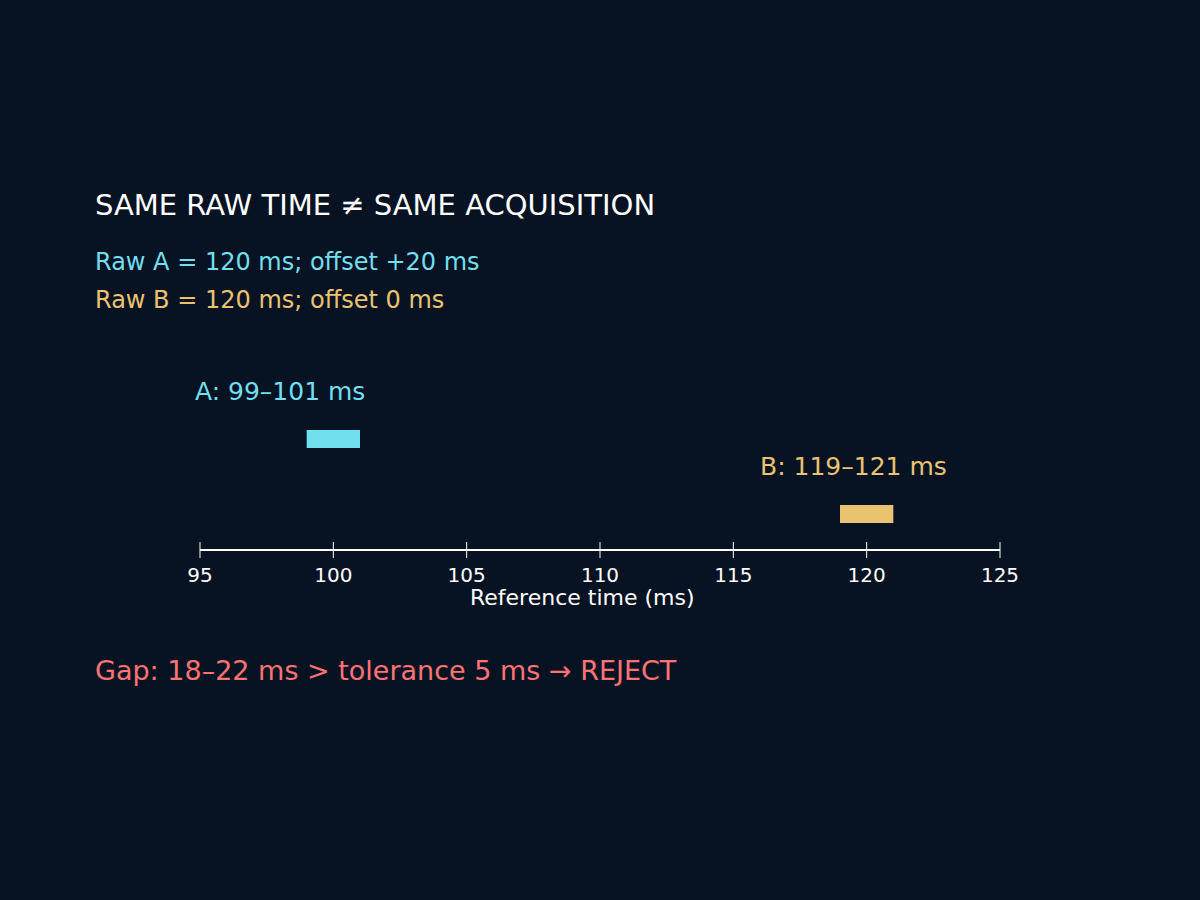
In the illustrated false-match case, both raw timestamps are 120 ms. Source A is known to be 20 ms ahead, so its corrected interval is [99, 101] ms; B is [119, 121] ms. The possible separation is 18–22 ms, outside the five-millisecond tolerance. Equal raw timestamps are therefore the wrong join key. The diagram uses a synthetic common epoch, not a measurement from an installed plant.
For a stream implementation, first select candidates using normalized intervals and a bounded search horizon. Then apply quality, epoch, freshness and temporal admissibility gates. If multiple candidates pass, use a documented sequence/one-to-one matching rule or declare ambiguity. This pairwise gate does not solve global matching, prevent sample reuse or prove causal association. Never select the raw nearest neighbour first and discard all alternatives before validating time.
Executed fixture: drift, holdover, steps and stale values
The fixture uses integer milliseconds and independent pairs from two synthetic streams. Each record retains its ground-truth acquisition instant solely for scoring, raw timestamp, offset estimate, uncertainty and validity. The classifier cannot access ground truth. Valid records are checked to contain that truth inside their declared interval. Clock-step and stale-value records are explicitly invalidated rather than allowed to hide outside an inaccurate interval.
| Synthetic case | Possible gap (ms) | Decision |
|---|---|---|
| Aligned | 0–4 | accept |
| False equal stamp | 18–22 | reject |
| Tracked drift | 0–5 | accept |
| Holdover | 0–18 | indeterminate |
| Clock step | — | invalid |
| Stale value | — | invalid |
| Tolerance edge | 1–5 | accept |
| Ambiguous outside | 2–10 | indeterminate |
For tracked drift, source B’s offset has moved to eight milliseconds and the current estimate tracks it with a two-millisecond uncertainty. Holdover instead widens both uncertainties to eight milliseconds. A separate arithmetic check models bound growth as u(age) = u0 + drift_bound × age: an illustrative 200 ppm bound adds four milliseconds over twenty seconds to an initial one millisecond. This is a chosen envelope, not a measured oscillator specification. Real temperature, aging, asymmetric paths and reference failure can invalidate it.
The clock-step case changes the raw clock by 100 ms while keeping the obsolete estimate; the record is invalid because the step detector has already raised a fault. This does not test step detection. A missed step could violate the bound and defeat the gate. The stale-value case likewise assumes a failed freshness/acquisition contract, not a rule that every unchanged OPC UA value is stale. Test those detectors against instrument evidence separately.
The raw rule accepts abs(rawA − rawB) ≤ 5 ms. It accepts four of eight proposed pairs, one falsely. The interval rule accepts three of eight and no false pair; it rejects one, abstains on two and invalidates two. Among five ground-truth-aligned pairs, it retains three: 60% coverage. One aligned pair is lost to holdover uncertainty and one to the invalid clock-step record. These small counts describe this constructed fixture only, not precision estimates for a deployment.
A separate nearest-neighbour negative control gives A a true time of 100 ms and raw time of 120 ms. B offers samples at true/raw times 120 and 102 ms. Raw nearest matching picks 120; the calibrated interval gate admits 102. Exact-boundary checks accept a zero-uncertainty gap of five milliseconds and reject six. The fixture is a deterministic policy test, not a PTP network, OPC UA server or acquisition-hardware test.
Implementation and operational release checklist
1. Agree the feature’s physical tolerance and acquisition semantics with instrumentation and process owners. Separate instantaneous samples from averages, filtered outputs and last-change notifications. Include filter delay when relevant; sensor downsampling and aliasing controls address bandwidth and causal delay rather than clock agreement.
2. Version raw-to-reference mapping, offset sign, units, calibration age, epoch and uncertainty provenance. Reject unavailable mappings; do not replace a missing source time with receipt time under the same field name. Keep the rejected record and reason in a bounded evidence store.
3. Monitor bound validity and expand uncertainty during holdover only under a justified drift model. Invalidate on detected steps, reference changes or expired calibration. Recovery needs evidence that the new epoch is calibrated, not merely a green synchronization indicator.
4. Apply the gate before feature assembly. Preserve input IDs, corrected intervals, policy version and reason codes with each accepted or declined pairing. Use bounded candidate buffers and explicit expiry; wider uncertainty increases both ambiguity and buffering pressure.
5. Test equality boundaries, offset-sign mistakes, missing timestamps, drift, clock steps, stale values, multi-candidate ambiguity, sequence reuse and domain conversion. This article executes the listed pairwise and nearest-time cases; device behavior, restart recovery and matching policy still require integration tests.
6. Report accepted, misaligned, indeterminate and invalid counts against all candidate pairs, plus per-sensor coverage and evidence age. Where ground truth exists, also report false accepts and retained aligned pairs. In live operation, do not label a rejected pair a verified physical error when truth is unknown.
Keep late-data feature finalization separate: watermarks and retention decide when a result may change, not whether its source clocks agree. Arrival delay, sampling aliasing and clock uncertainty are three different failure modes. Fixing one does not repair the others.
What this gate costs—and where to start
Conservative bounds reduce usable coverage and can bias which operating regimes reach the model. Holdover during a difficult operating condition may remove exactly the observations you need. Monitor missingness by asset and state, validate training/serving parity, and design an explicit abstention path instead of silently widening tolerance to recover attractive dashboards. A stricter gate cannot create missing acquisition evidence or establish causality, safety or regulatory compliance.
For an implementation review, bring one feature pair, producer timestamp documentation, a read-only trace and the physical tolerance you need to defend. I can help turn those into a versioned clock-domain contract, executable rejection tests and a coverage report. The first useful result is not “our clocks are synchronized”; it is a reproducible answer to which feature pairs your evidence actually permits.