
BLUF: A visual-inspection score is not automatically a defect probability, and a calibrated probability is not automatically a reject instruction. Separate three artifacts: the model that ranks inspected parts, the calibrator that maps scores to probabilities under a defined production distribution, and the decision policy that chooses accept, review or reject. Approve that policy against defect escapes, unnecessary scrap and available review capacity—not a default confidence threshold.
This article addresses part-level visual quality decisions, not predictive-maintenance alarm thresholds. The implementation below is a proposed engineering pattern grounded in scikit-learn documentation. All monetary values and plotted probabilities are illustrative assumptions, not factory measurements, customer results or recommended production settings. Safety-critical inspection requires separate domain validation and applicable conformity review.
Define what the score means before calibrating it
Start with a binary target: a part is nonconforming under a named inspection specification, based on a defined adjudication procedure. Record defect type and severity separately. A cosmetic blemish and a structural crack should not share an undifferentiated escape cost. If the model emits pixel anomaly scores, a bounding-box confidence or image similarity, do not label that output “probability that this part is defective.” First define and freeze how images, views and detections combine into one part-level score.
A maximum across multiple views changes the score distribution. Changing the camera count, crop policy or aggregation rule therefore changes the calibration problem even when model weights stay fixed. Bind the calibrator to the complete preprocessing and aggregation pipeline. Keep all images of one part together in evaluation; otherwise the test can reward recognition of the same surface rather than generalisation to another part.
The predictive-maintenance reference architecture provides the broader pattern of acquisition, context, scoring and outcome feedback. Here the independent decision unit is the inspected part, and the outcome is conformance—not a future maintenance event.
Build separate evidence for fitting, calibration and policy selection
Use model-training data, independent calibration data, a policy-validation set and a final acceptance set. This four-way separation is a conservative design recommendation, not a requirement to waste scarce labels on equally sized partitions. With limited data, nested, group-aware cross-validation can reuse development observations, but every probability used to select a policy must come from a properly held-out prediction path. Preserve one untouched acceptance evaluation.
Group by the strongest relevant dependence: part identity, production lot or acquisition session. For a claim about later production, also hold out a later period. The official GroupKFold documentation guarantees non-overlapping groups; it does not guarantee chronological training. A lot identifier alone cannot prevent future images from entering a training fold.
Audit class support in every fold. A fold with no defects cannot substantiate performance on defects. Deliberately enriching a dataset with bad parts helps challenge detection, but a calibrator fitted to that enriched mix does not automatically estimate probabilities at the live defect prevalence. Retain representative production sampling or a justified sampling-correction procedure. Report the challenge set separately from the prevalence-representative acceptance set.
The calibration guide recommends fitting the calibrator on data independent of classifier training. Its sigmoid method offers a constrained mapping; isotonic regression offers more flexibility but can overfit with insufficient data. Select between them using held-out evidence, not the impression that a flexible curve must be more accurate. Check the installed library version before adopting a particular API or method.
Read a reliability diagram, not just one loss number
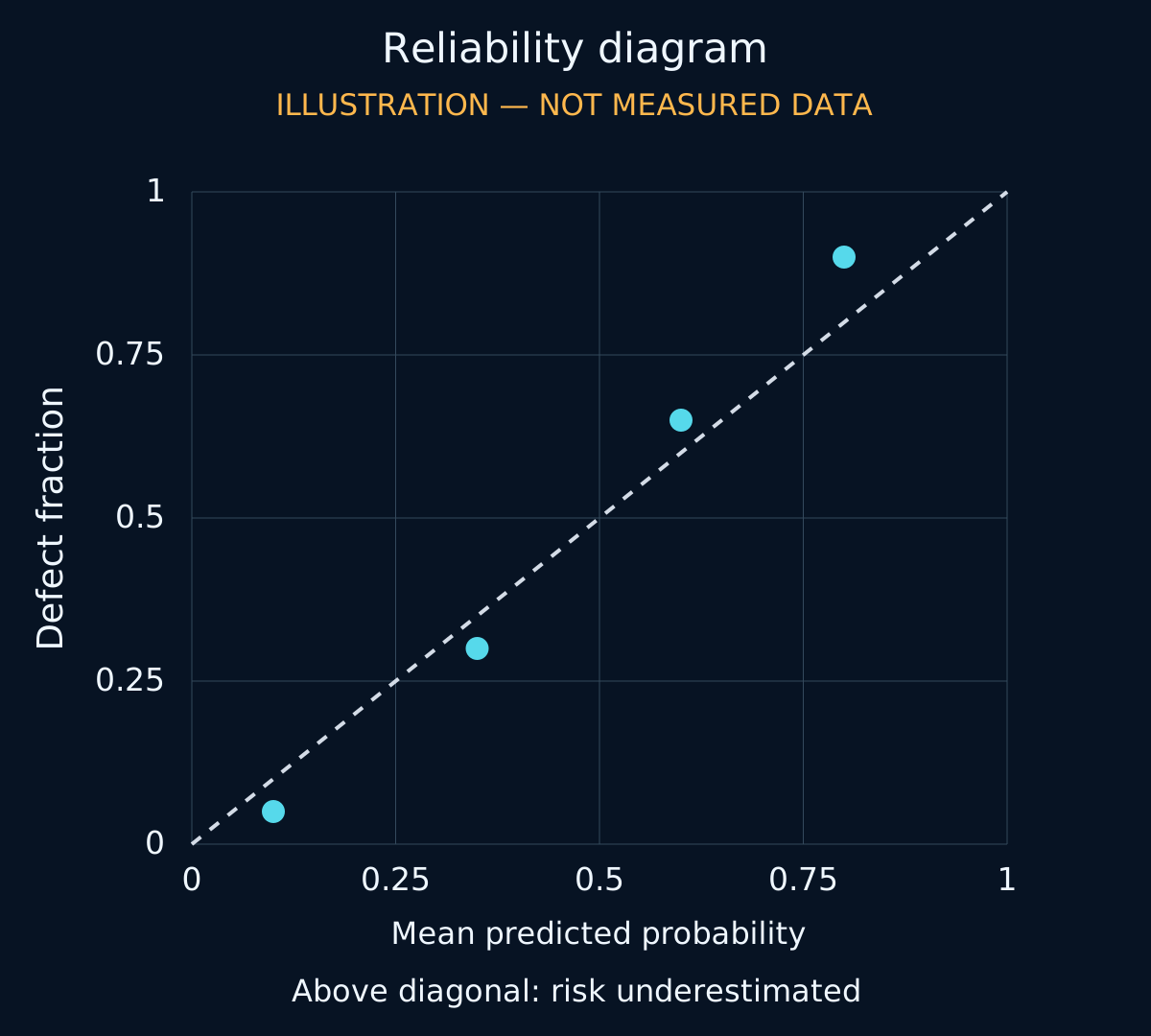
In a reliability diagram, the horizontal coordinate is the mean predicted defect probability in a bin and the vertical coordinate is the observed defect fraction in that bin. A point above the diagonal means that the model underestimates defect frequency in that range; a point below it means overestimation. Show bin counts alongside the curve. Empty or tiny bins do not become reliable because a line connects them.
The accompanying diagram uses deliberately hypothetical coordinates to teach this reading rule; it is not evidence that any calibration method improved an inspection model. For a real report, plot held-out raw and calibrated predictions on the same parts, retain the binning policy, and include uncertainty appropriate to lot-level dependence. Inspect the low-probability region around the accept boundary separately: a full-range chart can hide the region that controls defect escapes.
The official probability-calibration guide explicitly warns that Brier loss mixes reliability, resolution and uncertainty. Lower Brier loss alone does not prove better calibration. Report reliability curves, sample and defect counts, Brier loss or log loss, and discrimination metrics together. Global calibration can also conceal a bad camera or product variant; stratify the same checks by the deployment conditions you intend to approve.
Translate conformance errors into a decision table
Let p denote the calibrated probability of a defective part within the validated operating scope. For illustration, assume accepting a defective part costs €500, rejecting a conforming part costs €20, and manual review costs €3. Correct accept and correct reject actions have zero incremental cost relative to the chosen baseline. The example assumes a perfect reviewer who then routes the part correctly; real reviewers are neither free of errors nor infinitely available.
| Action | Cost if conforming | Cost if defective | Expected incremental cost |
|---|---|---|---|
| Accept | €0 | €500 escape cost | 500 × p |
| Review, idealised | €3 | €3 | 3 |
| Reject | €20 unnecessary scrap | €0 baseline | 20 × (1 − p) |
This is an action-by-truth cost matrix, not an observed confusion matrix. If rejecting a truly defective part incurs additional handling or disposal cost, add it to the defective column and recompute. Use the same economic boundary for every cell: warranty exposure, downstream rework and containment costs must not be counted twice. Quality and finance owners should approve the assumptions; data science should not invent the exchange rate between escapes and scrap.
Without review, the two losses are equal when 500p = 20(1 − p), giving p = 20/520, approximately 3.85%. With the idealised reviewer, the accept/review boundary is 3/500 = 0.6%, and the review/reject boundary is 1 − 3/20 = 85%. These wide review limits are a consequence of the deliberately cheap, perfect reviewer assumption—not a sensible default for an industrial line.
| Condition | Illustrative least-cost action | Operational precondition |
|---|---|---|
| p below 0.6% | Accept | Valid scope and approved escape-risk limit |
| p from 0.6% through 85% | Review | Reviewer available; ties assigned to review |
| p above 85% | Reject | Approved reject route and part traceability |
| Invalid image or unapproved product | Hold outside the cost rule | Apply the documented quality contingency |
At p = 2%, accept costs €10 in expectation, ideal review €3 and reject €19.60. The least-cost action is review, even though a default binary classifier would usually predict the non-defective class. The threshold-tuning guide makes this separation between probability estimation and action explicit. Its binary threshold tools do not by themselves implement a capacity-constrained three-action inspection policy.
Make the review queue part of the policy
Replace the ideal review loss with an operational model. If e_miss is the review miss probability conditional on a truly defective reviewed part, and e_scrap is the erroneous rejection probability conditional on a conforming reviewed part, the illustrative loss becomes 3 + 500p × e_miss + 20(1 − p) × e_scrap. Estimate these errors on the parts that enter review; the ambiguous subset may be harder than a random sample. Include delay or containment costs when they matter.
Capacity can dominate economics. At an illustrative throughput of 6,000 parts per hour, a 4% review share creates 240 reviews per hour. At 45 seconds each, that is three reviewer-hours per clock hour before breaks, handling and variability. A policy that looks inexpensive offline can therefore accumulate an unbounded queue. Measure arrivals, service time, queue age and disposition deadline in shadow operation.
Do not quietly widen automatic acceptance when the queue fills. Define a contingency with the quality owner: hold affected output, use an approved secondary inspection route or reduce throughput. A simple cost model must remain subordinate to mandatory quality constraints and the separately engineered line-control boundary. The alarm-rationalisation article explains a related attention-capacity problem, but inspection review needs part disposition and traceability rather than alarm deduplication.
Release workflow and acceptance checklist
The operating flow is: identify part and inspection specification → verify image quality and approved camera/product regime → compute frozen part-level score → apply matched calibrator → evaluate action costs and quality constraints → accept, queue for review or reject → record final adjudication. An invalid input branches to hold before the probability-based policy. A review timeout follows the quality contingency, not an implicit accept branch.
Checkpoint 1 — Freeze the bundle: model, preprocessing, multi-view aggregation, calibrator, policy, cost assumptions, approved product/camera scope and rollback target. Log the bundle ID with each decision, not just the model version.
Checkpoint 2 — Replay the complete decision policy on untouched acceptance lots. Produce an observed action-by-truth matrix: conforming and defective parts accepted, reviewed and rejected. Show totals, defect escapes among accepted parts, unnecessary scrap among conforming parts and review share among all eligible parts. Evaluate final reviewer dispositions as well as initial routing.
Checkpoint 3 — State denominators and exclusions. Missed-defect rate uses all truly defective eligible parts; defect contamination among accepted output uses accepted parts. They answer different questions. Keep uninspectable parts and pending labels visible. A zero observed escape count is not proof of zero risk, especially with few defects.
Checkpoint 4 — Test invalid images, camera replacement, lighting drift, unseen finishes, missing part identity, a full review queue and delayed ground truth. Verify that the intended hold or degraded path is enforced and that operators can reconcile every part. Do not tune the thresholds on the final acceptance failures and then call the same set independent evidence.
Checkpoint 5 — Audit some accepted parts using a sampling plan that supports the desired estimates. Labels obtained only from rejects and reviews create selective feedback and hide accepted defects. Preserve sampling probabilities where weighting is needed, and include delayed downstream findings without silently rewriting earlier reports.
Limits and a practical starting point
Calibration holds only relative to the data distribution and target definition used to establish it. Lighting changes, new materials and shifts in defect prevalence can invalidate the mapping. Recalibration cannot repair an inspection model that no longer separates good and bad parts, nor can a threshold cure inconsistent labels. Freeze consequential use outside the approved envelope until evidence supports restoration.
Start with one product family, one conformance definition and one explicit disposition decision. Bring lot-level image identities, adjudicated outcomes, current scrap and escape assumptions, and reviewer service-time observations. I can help turn these into a calibration report, tested decision policy and release checklist. The first useful result may be that labels or review capacity are insufficient; finding that before enabling automatic rejection is a defensible engineering outcome.